
Building the Sea Link in 3D
How we built a procedural bridge, skyline and open-top bus, then brought them to life with route animation, camera rigs, sunset and water in WebGL.
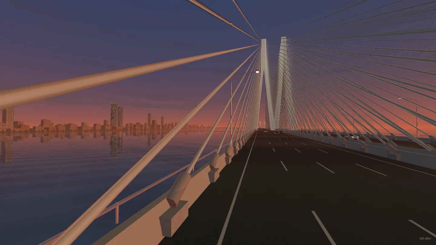
The Sea Link scene has to work from several very different viewpoints. From across the water, the pylons and cable fans carry the image. From the upper deck of the bus, you notice the road surface, barriers, seats and buildings passing beside you. A model that looks convincing in one distant render can fall apart when the camera moves through it.
We built the Sea Link experience in two parts. Python generates the bridge, coastline, skyline and vehicle as a GLB asset. A custom WebGL 2 renderer uses JavaScript and GLSL to animate the ride, position the cameras and draw the changing sky and water. This article follows that process from the first road coordinates to the final frame.
The scene is an artistic reconstruction. Its bridge remains rigid, its bus follows an authored route, and its waves are a shading effect. Here, simulation means prescribed motion and real-time rendering; the project does not calculate structural loads, cable tension, vehicle dynamics or fluid flow.
Jump to: Geometry · City and bus · Asset format · Motion and cameras · Light and water · Performance
Start with one road alignment
The most useful piece of the model is a function that says where the road is. Once that exists, lanes, barriers, pylons and moving objects can share a spatial reference.
The authoring scripts use X along the bridge, Y toward the coast and Z upward. A station parameter, s, runs from −1700 to 3000. The middle of the alignment is straight; circular approaches with radii of 850 and 1200 turn toward the land at either end. These are authored scene dimensions, not a surveyed map or a claim about the real bridge’s total length.
At each station, a tangent comes from sampling the path slightly before and after the point. Rotating that tangent by 90 degrees gives a lateral normal. In compact form, placement becomes:
T(s) = normalize(C(s + 0.01) - C(s - 0.01))
N(s) = (-T.y, T.x)
P(s, offset) = C(s) + offset * N(s)
Here, C is the two-dimensional centreline. Elevation is supplied separately. The main road sits near 24 units, with a small rise around the principal span:
h(s) = 24 + 1.8 * exp(-((s + 50) / 340)^2)Within 330 units of either endpoint, a smoothstep blend, t²(3−2t), brings that height down toward 4.5. The same height function later places the bus. That shared rule prevents the vehicle and road from disagreeing as the route rises and falls.
Two box-girder cross-sections, each 20 units wide, sit at offsets of −11 and +11. Connecting successive sections at three-unit intervals produces the deck shells. Asphalt strips, lane markings, swept concrete barriers and tubular rails follow the same alignment. Each carriageway has four lanes, with a two-unit separation between the decks.
This method makes a road edit propagate through the scene. Changing a bend does not require manually repositioning every stripe and barrier. It also keeps the construction understandable: an alignment, a cross-section and a sampling interval determine most of the deck geometry.
Build the pylons and stays from small primitives
The modeling vocabulary is deliberately small: boxes, tubes, chamfered columns and connected rings. A tube establishes a local frame along its centreline and places a polygonal cross-section at each sample. A chamfered column connects eight-point rings. Boxes provide the hard-edged pieces used throughout the bridge and city.
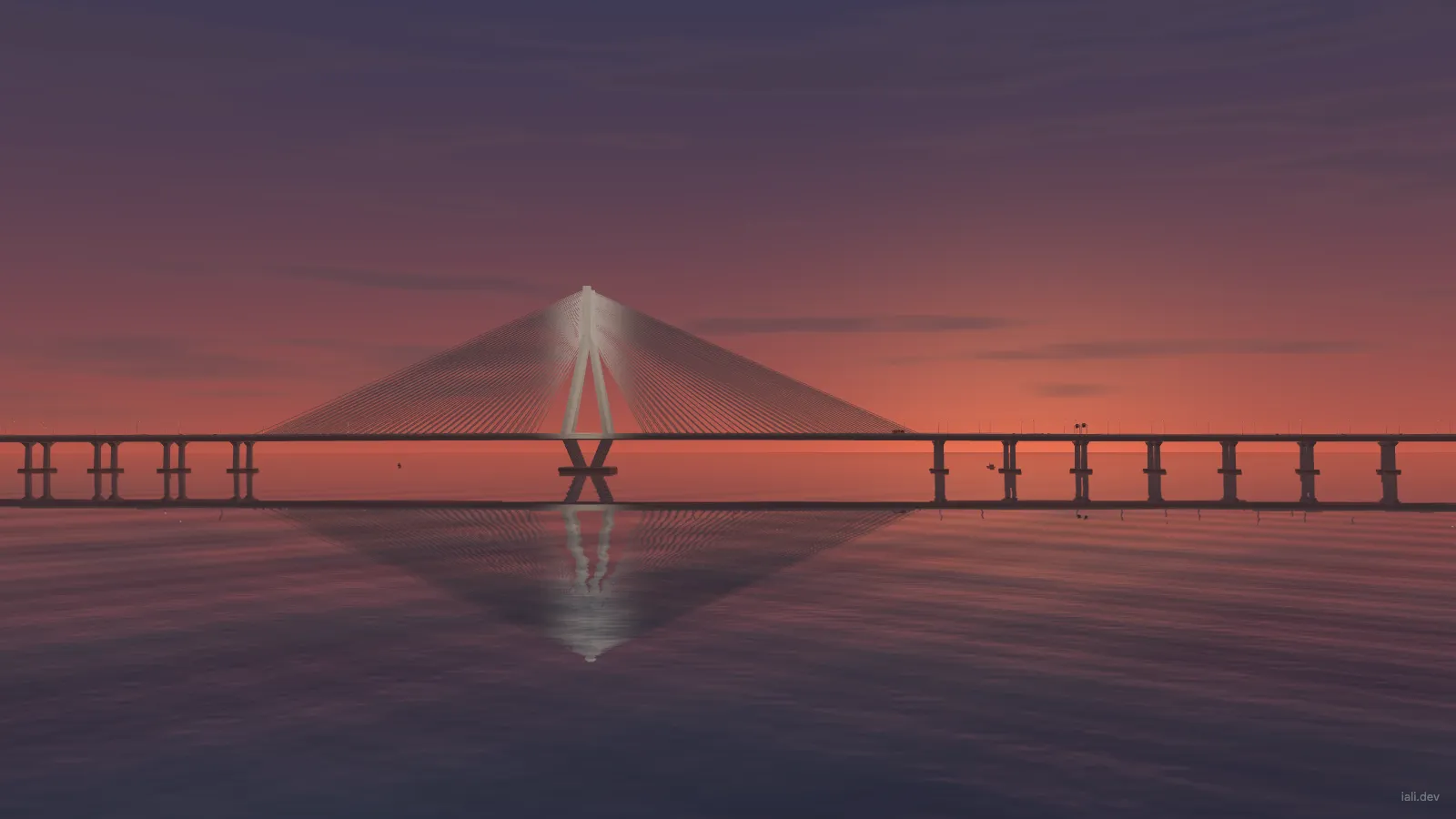
The main pylons use four chamfered legs that spread near deck level and converge toward the head. Their depth matters. A flat A-shaped silhouette might work from the front, but the moving camera needs a three-dimensional diamond form. Smaller pylons repeat the same general construction with different proportions.
For reference, the engineering account Making of Bandra–Worli Sea Link describes twin four-lane carriageways and 264 stays at Bandra plus 160 at Worli. The model uses that 424-stay split: two main pylons with 132 stays each, and four smaller pylons with 40 each. This anchors the recognizable structure while leaving the scene’s approaches and surroundings interpretive.
Each stay connects a deck anchor to a pylon anchor. A small parabolic adjustment gives it visible sag:
P(t) = (1 - t) * A + t * B
P.z -= 4 * sag * t * (1 - t)
The endpoints remain fixed; the maximum vertical adjustment occurs halfway along the cable. Main stays use a sag value of 0.13 and radius of 0.12; smaller stays use 0.025 and 0.10. Each cable has nine longitudinal samples and a six-sided cross-section. Separate anchor shoes finish the connections.
These values describe a visual curve. They are not the result of a catenary, tension or wind calculation. The distinction matters because procedural geometry can look precise without carrying engineering meaning.
Give the city depth without modeling every window
The surrounding city combines repeatable variation with a few deliberately composed tower groups. Seeded random choices vary the width, depth, height and position of low- and medium-rise buildings across six rows. Taller groups add floor bands, vertical fins, crowns and rooftop equipment. Four oval towers use twenty-sided plans.
The coastline is another authored function, combining broad sine and cosine terms with a local indentation. Rectangular exclusion regions reserve the bridge landfalls. This creates layers to look through from the bus: nearby masses move quickly across the view, while distant towers remain visible behind them.
Architectural references such as KPF’s Three Sixty West help establish the visual vocabulary of the Mumbai skyline. They do not make this a building survey. The modeled city is composed around the experience’s viewpoints, with simplified placement and proportions.
Much of the surface detail comes from small textures generated with Pillow. Concrete combines fine noise with enlarged coarse noise; asphalt uses RGB variation. Facades arrange rectangles and lines into window grids. The enhanced buildings use 512 × 1024 patterns with 32 rows and eight columns, varying glass and plaster colours. Signs and bus lettering are drawn with locally available fonts.
This gives the geometry detail at different distances without creating a mesh for every window. Reference photographs guide silhouettes and colour choices; their pixels are not embedded as textures by these modeling scripts.
Treat the bus as a hierarchy
The bus needs more detail than a distant vehicle because several cameras sit inside it. Its body includes segmented wheel arches, glazing on the lower deck, radiator details, destination lettering, seats, a boarding platform, steps and steering controls. The wheels are layered meshes attached to four pivot nodes beneath one bus root.
That hierarchy separates two kinds of movement. Transforming the root moves the entire bus through the world. Rotating a wheel pivot spins its child geometry around the axle without changing the placement of the body.
The open-deck revision changed the geometry itself. It removed the roof, upper glazing, frames and obstructing poles, and lowered the front fascia while retaining the seats and lower deck. This is why the upper camera can see ahead through a real opening. The vehicle is a fictional open-top adaptation, not a historical replica or a roadworthiness design.
The replacement script locates the existing bus root and wheel pivots, swaps their meshes, remaps material references and removes unused resources. It asserts that the animation data is preserved. The archived geometry check records zero upper-glass vertices, no obstruction in the tested front aperture and 76 unchanged environment mesh groups. Those checks make a focused bus revision less likely to disturb the bridge around it.
Package the scene for the renderer
Geometry accumulates in batches keyed by category and material. Before export, the builder welds identical position, normal, UV and colour tuples. Comparing the whole tuple preserves hard edges and texture seams that would disappear if vertices were merged by position alone. This is batching and deduplication; it does not use GPU instancing.
The exporter converts positions and normals from (x, y, z) to (x, z, −y), moving from the scripts’ Z-up coordinates to glTF’s Y-up convention. GLB keeps the mesh data and embedded images together. The glTF 2.0 specification defines that coordinate convention and binary container; the project adds category information in its own metadata.
The current delivered asset contains:
| Asset measure | Verified count |
|---|---|
| Active mesh nodes / primitives | 109 / 109 |
| Referenced vertices | 827,531 |
| Triangles | 483,111 |
| Materials / embedded images | 67 / 18 |
| Animation clips / channels | 1 / 6 |
| GLB bytes | 38,061,732 |
These are asset counts, not a frame-rate benchmark. The runtime replaces the model’s static water mesh with its own shader-driven surface. Opening the photo studio can add separate display geometry, so the GLB is not a complete count of everything the application may draw.
The browser loader is deliberately specific to this asset. It reads the mesh attributes, materials and embedded images needed by the renderer; it is not a general-purpose glTF implementation. That narrow scope keeps the format boundary small, but it also means an arbitrary GLB cannot be substituted without checking its features and layout.
Move the bus with a route function
The GLB includes a conventional six-channel animation: body translation, body rotation and four wheel rotations. The browser does not play those channels. It evaluates an analytic route in JavaScript instead, giving the ride controls direct access to distance, speed and pause state.
The route has four phases: travel along one carriageway, turn through a semicircle, return on the other carriageway, then turn again. The lane offsets and turnaround radius are 16.325 units. For the 4700-unit one-way station span, the loop parameter is:
loop = 2 * 4700 + 2 * pi * 16.325
     ≈ 9502.573
distance += dt * 11.667 * playbackSpeed
The base speed is labeled 42 km/h. It is nominal: the parameter follows road stations rather than integrated three-dimensional distance along each offset lane. Grade and curvature therefore affect the relationship between that label and the vehicle’s actual displacement. The turnaround loops are also part of the authored scene.
The route supplies position and heading. A finite difference of the road-height function supplies slope, and a curvature adjustment converts that slope into the body’s pitch along each lane. Turnarounds use zero pitch. Each wheel’s rotation comes from traveled route parameter divided by its 0.545 radius; the wheels do not have independent steering or suspension.
Frame intervals are capped at 0.05 seconds. When a hidden tab becomes visible again, timing restarts instead of advancing the bus through the entire absence. Pause stops route advancement while leaving camera controls usable.
Attach cameras to the ride
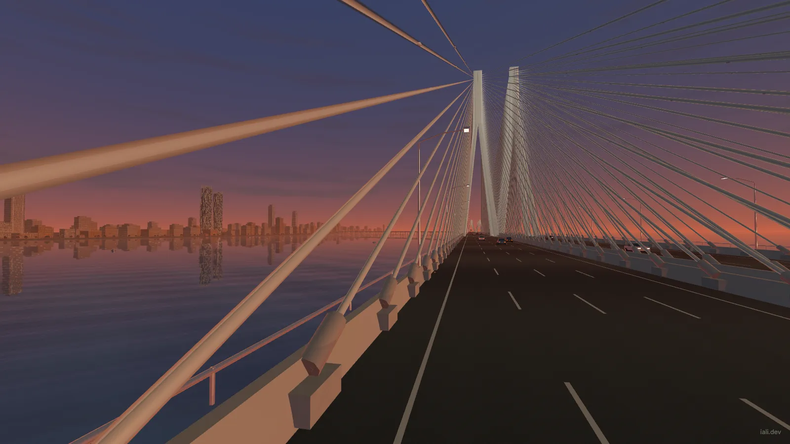
Most ride cameras define an eye and a target in bus-local coordinates. Applying the bus transform moves both into the world. The sea-facing view places its eye on the bus but builds its target from the world-space sun direction. Upper-deck and side-seat cameras attach directly, while chase and flyover views interpolate toward their desired positions.
The smoothing coefficient is time-based:
k = 1 - exp(-9 * dt)
eye = eye + k * (desiredEye - eye)
Using elapsed time keeps the smoothing response more consistent across different frame intervals. Seat views use a small 0.08 near plane so nearby bus geometry remains visible; the flyover camera can use a larger near plane. A subtle sine-based bob adds motion to seated views while the ride is running.
The sea-facing camera also considers the sun direction. It chooses the appropriate side of the bus and aims toward the sunset as the vehicle changes heading. The camera’s purpose stays recognizable on both legs of the trip.
Dragging, scrolling or using camera keys detaches from the bus and turns the current eye and target into a free orbit. The bus keeps going. Preserving the current view during that transition avoids a jump back to an unrelated preset.
Drive the sunset from shared state
The sunset control interpolates between four lighting keyframes. Each specifies sun elevation, direct power, ambient contribution, night contribution and colours for the sky and water. The authored elevation moves from +7 degrees to −3.8 degrees, while the horizontal direction remains fixed.
The sky shader combines a horizon-to-zenith gradient, warmth toward the sun, noise-based clouds, a low haze bank and an angular sun disc. The disc’s diameter is approximately 0.53 degrees, with a softened edge. This timeline is art direction, not a clock-driven astronomical calculation or a weather model.
The useful connection is shared state. The sky, surface lighting and water highlights read the same sun direction. The shadow camera derives its direction from that state, with its elevation clamped just above the horizon. Moving one slider therefore changes a coherent scene rather than several unrelated colour effects.
Opaque surfaces use metallic and roughness parameters with a GGX-style microfacet distribution and Schlick-style approximations. Ambient light, reflected sky, distance fog and a tone curve complete the image. This is physically inspired real-time shading with several deliberate approximations.
Shadows come from one 2048 × 2048 depth map and a fixed orthographic light view. The renderer refreshes it when lighting changes, then reuses it. Its selected shadow geometry excludes the moving bus, cables and skyline, among other categories. That bounds the shadow work, at the cost of those objects not casting dynamic shadows.
Make water from a plane and a second view
The sea’s surface is two triangles. Its vertices stay on the water plane; the apparent waves come from the fragment shader.
Several sine components and moving noise layers define a height field. Sampling nearby points produces a surface normal. Higher frequencies fade according to their screen-space footprint, reducing distant shimmer. The wind control changes the wave amplitude used in this shading calculation.
To reflect the bridge, the renderer mirrors the camera’s eye and target across Y = 0 and renders another view into a 1024 × 640 texture. The water shader samples that texture with coordinates distorted by the wave normal. A Fresnel term gives the reflection more weight at grazing angles; sunlight adds a glitter path and smaller highlights.
The frame follows this order:
Refresh the shadow map when dirty
  → Render reflected sky, scene and photo lights
  → Draw the main sky and opaque geometry
  → Draw water using the reflection texture
  → Draw transparent geometry and photo lights
Because the reflection pass draws the scene again, the bus and applied photo lights appear in it as they change. This is a planar reflection with surface distortion. It does not trace rays through waves or calculate wakes and shoreline flow. Its main cost is the extra scene render on every rendered frame.
Spend detail where the camera can use it
Thin cables are a particular problem. At a distance, a correctly sized tube may cover less than a pixel and flicker or vanish. The vertex shader widens distant stays toward a minimum screen-space coverage, while reducing their opacity to compensate. Their silhouette remains readable without pretending that the exported cable radius has changed.
Static buffers and vertex-array objects are uploaded once. Materials and draw lists are prepared ahead of rendering, uniform locations are cached, and consecutive redundant material binds are avoided. Texture mipmaps help with shrinking detail. These choices follow the broader principle in MDN’s WebGL best practices: reduce avoidable draw and state-management work.
The main drawing buffer is capped at roughly 2.4 million pixels, with device-pixel-ratio limits of 1.5 for ordinary pointers and 1.25 for coarse pointers. Shadow and reflection targets keep their fixed sizes. The scene has no general level-of-detail or per-building visibility system, so pixel limits do not eliminate its geometry and reflection costs.
Hidden pages stop rendering. Reduced-motion preferences initially pause the ride and sunset, freeze ambient water motion and let unchanged frames skip GPU redraws. If the WebGL context is lost, retained geometry and image data let the renderer recreate its resources; the applied photo is restored separately from any unfinished draft. Keeping those CPU-side copies aids recovery but also uses memory.
Keep the build inspectable
The procedural generators use fixed random seeds, making their choices repeatable under the same execution path. Fonts are an external input: different local font availability can change lettering and texture bytes. A seed alone does not guarantee identical output across machines.
We checked the current asset’s mesh, triangle, material and animation counts, and preserved the focused geometry checks from the open-deck replacement. The later packaging audit verified the existing model bytes and an isolated viewer build; it did not regenerate the entire historical modeling chain. That distinction keeps a successful packaging check from becoming an unsupported claim about full reproducibility.
The scene works because its pieces share a few explicit rules: road alignment places the bridge and bus, the bus transform carries the cameras, and the sun direction connects sky, surfaces and water. Each system remains small enough to inspect, while the relationships between them make the ride feel continuous.
Explore the scene
Open the ride, switch between an upper-deck seat and a view across the water, then move the sunset control. Those changes reveal the geometry, camera and reflection techniques described here.
Open Sea Link · Read how the photo studio works · Project story
The companion photo-studio article covers image preparation, cable-fan textures and PNG capture. Personal, non-commercial scene captures are permitted under the model and image-use terms; model reuse and commercial use require separate permission.